9 Eigenvalues and eigenvectors

Eigenvalue problems are among the most important problems in linear algebra, and they occur throughout quantum chemistry. In an eigenvalue problem, we are given a square matrix $A\in\mathbb{C}^{n\times n}$ and seek a number $\lambda\in\mathbb{C}$ and a nonzero vector $\mathbf{x}\in\mathbb{C}^n$ such that

\[ A\mathbf{x}=\lambda\mathbf{x}. \]

The number $\lambda$ is called an eigenvalue of $A$, and the nonzero vector $\mathbf{x}$ is called an eigenvector corresponding to $\lambda$. In column-vector notation,

\[ \mathbf{x}=\begin{bmatrix}x_1\\x_2\\\vdots\\x_n\end{bmatrix}. \]

The equation $A\mathbf{x}=\lambda\mathbf{x}$ says that multiplication by $A$ has a particularly simple effect on an eigenvector: it only multiplies the vector by a number. Thus, the direction represented by $\mathbf{x}$ is left unchanged, apart from multiplication by the scalar $\lambda$. Notice that $\mathbf{x}=\mathbf{0}$ is excluded from the definition, since $A\mathbf{0}=\lambda\mathbf{0}$ holds for every $\lambda$ and therefore tells us nothing about the matrix.

The eigenvalue equation can equivalently be written as

\[ (A-\lambda I)\mathbf{x}=\mathbf{0}, \]

where $I$ is the identity matrix. Since we require $\mathbf{x}\neq\mathbf{0}$, the matrix $A-\lambda I$ must have a nontrivial null space and therefore cannot be invertible. For a finite-dimensional square matrix, this is equivalent to

\[ \det(A-\lambda I)=0. \]

This equation is called the characteristic equation or secular equation of $A$. Its solutions are the eigenvalues of $A$. Once an eigenvalue $\lambda$ has been found, the corresponding eigenvectors are obtained by solving the homogeneous linear system $(A-\lambda I)\mathbf{x}=\mathbf{0}$.

An especially important situation occurs when $A$ has enough linearly independent eigenvectors to form a basis of $\mathbb{C}^n$. Suppose these eigenvectors are

\[ \mathbf{x}_1,\mathbf{x}_2,\ldots,\mathbf{x}_n, \]

where the subscript labels the different vectors. Thus,

\[ \mathbf{x}_j= \begin{bmatrix} x_{1j}\\ x_{2j}\\ \vdots\\ x_{nj} \end{bmatrix} \]

denotes the $j$’th eigenvector, while $x_{ij}$ denotes its $i$th component. If $\mathbf{x}_j$ has eigenvalue $\lambda_j$, then

\[ A\mathbf{x}_j=\lambda_j\mathbf{x}_j,\qquad j=1,\ldots,n. \]

We can collect these eigenvectors as the columns of a matrix

\[ X=[\mathbf{x}_1\ \mathbf{x}_2\ \cdots\ \mathbf{x}_n] \]

and collect their corresponding eigenvalues in the diagonal matrix

\[ D=\begin{bmatrix} \lambda_1 & 0 & \cdots & 0\\ 0 & \lambda_2 & \cdots & 0\\ \vdots & \vdots & \ddots & \vdots\\ 0 & 0 & \cdots & \lambda_n \end{bmatrix}. \]

The $n$ separate eigenvalue equations can then be written as the single matrix equation

\[ AX=XD. \]

Because the eigenvectors form a basis, $X$ is invertible. Consequently,

\[ A=XDX^{-1}. \]

A matrix for which such an eigenvector basis exists is called diagonalizable. Diagonalization is useful because the action of a diagonal matrix is particularly simple: it acts independently on each component. In a basis of eigenvectors, the matrix $A$ therefore has its simplest possible form. This idea is fundamental in quantum mechanics, where many important matrices, in particular Hermitian matrices, possess an orthonormal basis of eigenvectors.

In the exercises below, we study how eigenvalues and eigenvectors are found, when a matrix can be diagonalized, and why Hermitian and, more generally, normal matrices have especially useful eigenvalue decompositions.

Exercises

Exercise 9.1 (Checking candidate eigenvectors) Consider the real symmetric matrix

\[ A=\begin{bmatrix} 2 & 1\\ 1 & 2 \end{bmatrix}. \]

Recall that a nonzero vector $\mathbf{x}$ is an eigenvector of $A$ if

\[ A\mathbf{x}=\lambda\mathbf{x} \]

for some number $\lambda$. In other words, after multiplication by $A$, the vector must point in the same or exactly opposite direction: it may be stretched, compressed, or multiplied by a negative number, but its direction cannot otherwise change.

For each of the following candidate vectors, compute $A\mathbf{x}$ and decide whether $\mathbf{x}$ is an eigenvector of $A$. If it is, find the corresponding eigenvalue $\lambda$.

Consider

\[ \mathbf{x}=\begin{bmatrix}1\\1\end{bmatrix}. \]

Compute $A\mathbf{x}$. Can the result be written as $\lambda\mathbf{x}$? If so, what is $\lambda$?
Consider

\[ \mathbf{x}=\begin{bmatrix}1\\-1\end{bmatrix}. \]

Compute $A\mathbf{x}$ and determine whether $\mathbf{x}$ is an eigenvector. If it is, find its eigenvalue.
Consider

\[ \mathbf{x}=\begin{bmatrix}1\\0\end{bmatrix}. \]

Compute $A\mathbf{x}$. Is the result a scalar multiple of $\mathbf{x}$? Is $\mathbf{x}$ an eigenvector?
Consider

\[ \mathbf{x}=\begin{bmatrix}2\\2\end{bmatrix}. \]

Without doing the full matrix-vector multiplication at first, compare this vector with the vector in part a. Do you expect it to be an eigenvector? Check your answer by computing $A\mathbf{x}$.
The vectors in parts a and d are different vectors, but they point in the same direction. What eigenvalue do they have? What does this tell you about scalar multiples of an eigenvector?
Compare the two eigenvectors found in parts a and b. Compute their ordinary dot product. What do you observe?

Exercise 9.2 (Eigenvalues in chemical kinetics) Consider the reversible reaction

\[ \mathrm{A}\underset{k}{\stackrel{k}{\rightleftharpoons}}\mathrm{B}. \]

The positive number $k$ is called the rate constant. It tells us how rapidly the reaction takes place. Here we use the same rate constant for the forward reaction $\mathrm{A}\to\mathrm{B}$ and the backward reaction $\mathrm{B}\to\mathrm{A}$, to keep the example simple.

Let $a(t)$ and $b(t)$ denote the concentrations of A and B. For a first-order reaction, the reaction rate is proportional to the concentration of the reacting species. Thus, A is converted into B at a rate $ka$, while B is converted into A at a rate $kb$. The larger $k$ is, the faster the reaction proceeds. If concentration is measured in $\mathrm{mol\,L^{-1}}$ and time in seconds, $k$ has units of $\mathrm{s^{-1}}$.

The concentration of A therefore decreases due to the forward reaction at a rate $ka$ and increases due to the backward reaction at a rate $kb$. Similarly, the concentration of B increases at a rate $ka$ and decreases at a rate $kb$. This gives the rate equations

\[ \frac{da}{dt}=-ka+kb,\qquad \frac{db}{dt}=ka-kb. \]

If we collect the concentrations in the vector

\[ \mathbf{x}(t)=\begin{bmatrix}a(t)\\b(t)\end{bmatrix}, \]

the rate equations can be written as

\[ \frac{d\mathbf{x}}{dt}=K\mathbf{x},\qquad K=\begin{bmatrix}-k&k\\k&-k\end{bmatrix}. \]

We will see that the eigenvectors of $K$ describe two particularly simple ways in which the concentrations can change.

Consider the vector

\[ \mathbf{x}_1=\begin{bmatrix}1\\1\end{bmatrix}. \]

Calculate $K\mathbf{x}_1$ and show that $\mathbf{x}_1$ is an eigenvector of $K$. What is its eigenvalue? Explain chemically why nothing changes when $a=b$.
Now consider

\[ \mathbf{x}_2=\begin{bmatrix}1\\-1\end{bmatrix}. \]

Calculate $K\mathbf{x}_2$ and show that it is also an eigenvector. What is its eigenvalue?
Suppose that the concentration vector has the form

\[ \mathbf{x}(t)=c(t)\mathbf{x}_2. \]

Insert this into the rate equation and use your result from part b to show that

\[ \frac{dc}{dt}=-2kc. \]

Thus $c(t)=c(0)e^{-2kt}$. What happens to this contribution as time increases? What happens more rapidly if the rate constant $k$ is increased? Explain why the two eigenvectors $\mathbf{x}_1$ and $\mathbf{x}_2$ can be interpreted as an equilibrium mode and a relaxation mode, respectively.

Exercise 9.3 (Eigenvalues and diagonalization of a Hermitian matrix) Consider the matrix

\[ A=\begin{bmatrix} 2 & -\mathrm{i}\\ \mathrm{i} & 2 \end{bmatrix}. \]

Show that $A$ is Hermitian, that is, verify that

\[ A^H=A. \]
The eigenvalues of $A$ are the values of $\lambda$ for which

\[ \det(A-\lambda I)=0. \]

Set up the matrix $A-\lambda I$, calculate its determinant, and find the two eigenvalues $\lambda_1$ and $\lambda_2$. Verify that both eigenvalues are real. (The determinant of $\begin{bmatrix} a & b \\ c & d \end{bmatrix}$ is $ad-bc$.)
For each eigenvalue $\lambda_j$, solve

\[ (A-\lambda_j I)\mathbf{x}_j=\mathbf{0} \]

to find a corresponding eigenvector $\mathbf{x}_j$. Normalize the eigenvectors so that

\[ \mathbf{x}_j^H\mathbf{x}_j=1. \]
Verify explicitly that your two normalized eigenvectors are orthogonal,

\[ \mathbf{x}_1^H\mathbf{x}_2=0. \]

Thus, the eigenvectors form an orthonormal basis of $\mathbb{C}^2$.
Form the matrix $U$ whose columns are the normalized eigenvectors,

\[ U=[\mathbf{x}_1\ \mathbf{x}_2]. \]

Show explicitly that $U$ is unitary by calculating $U^HU$.
Form the diagonal matrix

\[ D=\begin{bmatrix} \lambda_1&0\\ 0&\lambda_2 \end{bmatrix}, \]

where the ordering of the eigenvalues must agree with the ordering of the eigenvectors in $U$.
Verify by direct matrix multiplication that

\[ A=UDU^H. \]

Equivalently, verify that $U^HAU=D$. Explain briefly why $U^{-1}=U^H$ in this diagonalization.

Exercise 9.4 (A matrix that cannot be diagonalized) Consider the matrix

\[ A=\begin{bmatrix} 2 & 1\\ 0 & 2 \end{bmatrix}. \]

Find the eigenvalues of $A$ by solving the characteristic equation $\det(A-\lambda I)=0$. How many distinct eigenvalues does $A$ have?
Find all eigenvectors corresponding to the eigenvalue you found. How many linearly independent eigenvectors does $A$ have?
To diagonalize a $2\times2$ matrix, we need two linearly independent eigenvectors, which can be used as the columns of an invertible matrix $U$. Explain why this is impossible for $A$, and conclude that $A$ is not diagonalizable.

Exercise 9.5 (A reversible reaction with different rate constants) It is recommended that you first complete Exercise 9.2.

Consider now the more general reversible reaction

\[ \mathrm{A}\underset{k_b}{\stackrel{k_f}{\rightleftharpoons}}\mathrm{B}, \]

where $k_f>0$ is the rate constant for the forward reaction $\mathrm{A}\to\mathrm{B}$ and $k_b>0$ is the rate constant for the backward reaction $\mathrm{B}\to\mathrm{A}$. The concentrations satisfy

\[ \frac{d\mathbf{x}}{dt}=K\mathbf{x},\qquad \mathbf{x}(t)=\begin{bmatrix}a(t)\\b(t)\end{bmatrix},\qquad K=\begin{bmatrix}-k_f&k_b\\k_f&-k_b\end{bmatrix}. \]

Find the two eigenvalues of $K$ and a corresponding eigenvector for each eigenvalue. Show that one eigenvalue is zero and that the other is negative.
The eigenvector with eigenvalue zero describes an equilibrium concentration vector. Use it to show that at equilibrium

\[ \frac{b}{a}=\frac{k_f}{k_b}. \]

Explain why this result also follows directly by requiring the forward and backward reaction rates to be equal.
The other eigenvector describes relaxation toward equilibrium. Show that its time dependence contains the factor

\[ e^{-(k_f+k_b)t}. \]

What does this tell you about the rate at which the system approaches equilibrium?

Exercise 9.6 (Eigenvalues of a reaction network) It is recommended that you first complete or at least read through Exercise 9.2 and Exercise 9.5.

Consider the reaction network

\[ \mathrm{A}\underset{k_{BA}}{\stackrel{k_{AB}}{\rightleftharpoons}}\mathrm{B} \underset{k_{CB}}{\stackrel{k_{BC}}{\rightleftharpoons}}\mathrm{C}, \qquad \mathrm{B}\underset{k_{DB}}{\stackrel{k_{BD}}{\rightleftharpoons}}\mathrm{D} \underset{k_{ED}}{\stackrel{k_{DE}}{\rightleftharpoons}}\mathrm{E}. \]

All reactions are first order. Let

\[ \mathbf{x}(t)= \begin{bmatrix} a(t)\\ b(t)\\ c(t)\\ d(t)\\ e(t) \end{bmatrix} \]

contain the concentrations of the five species. Use the rate constants

\[ k_{AB}=1.0,\quad k_{BA}=0.4,\quad k_{BC}=0.7,\quad k_{CB}=0.2,\quad k_{BD}=0.5,\quad k_{DB}=0.3,\quad k_{DE}=0.8,\quad k_{ED}=0.1, \]

in units of $\mathrm{s}^{-1}$.

Write the five coupled rate equations and show that they can be written as

\[ \frac{d\mathbf{x}}{dt}=K\mathbf{x}. \]

Construct the $5\times5$ rate matrix $K$. Check that the sum of the components of $d\mathbf{x}/dt$ is zero. What quantity is therefore conserved?
Use Python to compute the eigenvalues and eigenvectors of $K$. You may use, for example,
```
import numpy as np

eigenvalues, eigenvectors = np.linalg.eig(K)
```
Identify the eigenvalue that is zero, up to numerical precision. Verify that all the other eigenvalues have negative real parts. What do the zero eigenvalue and the negative eigenvalues mean physically?
Scale the eigenvector belonging to the zero eigenvalue so that its components sum to $1$. Interpret the resulting components in terms of fractions of A, B, C, D, and E.
Start with all material in A,

\[ \mathbf{x}(0)= \begin{bmatrix} 1\\ 0\\ 0\\ 0\\ 0 \end{bmatrix}. \]

Compute

\[ \mathbf{x}(t)=e^{Kt}\mathbf{x}(0) \]

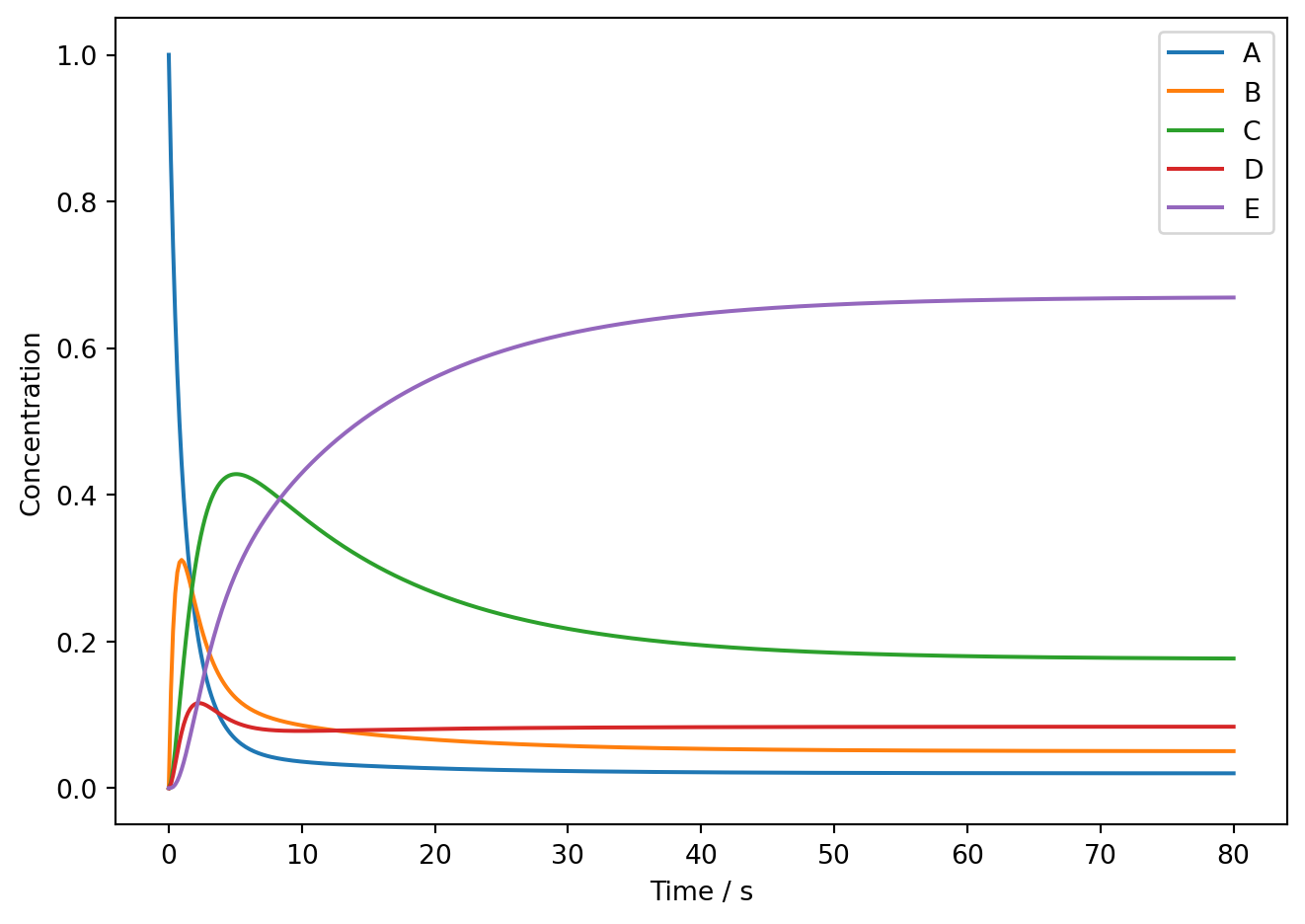
numerically for a suitable range of times. You may use scipy.linalg.expm to evaluate the matrix exponential. Plot all five concentrations as functions of time.

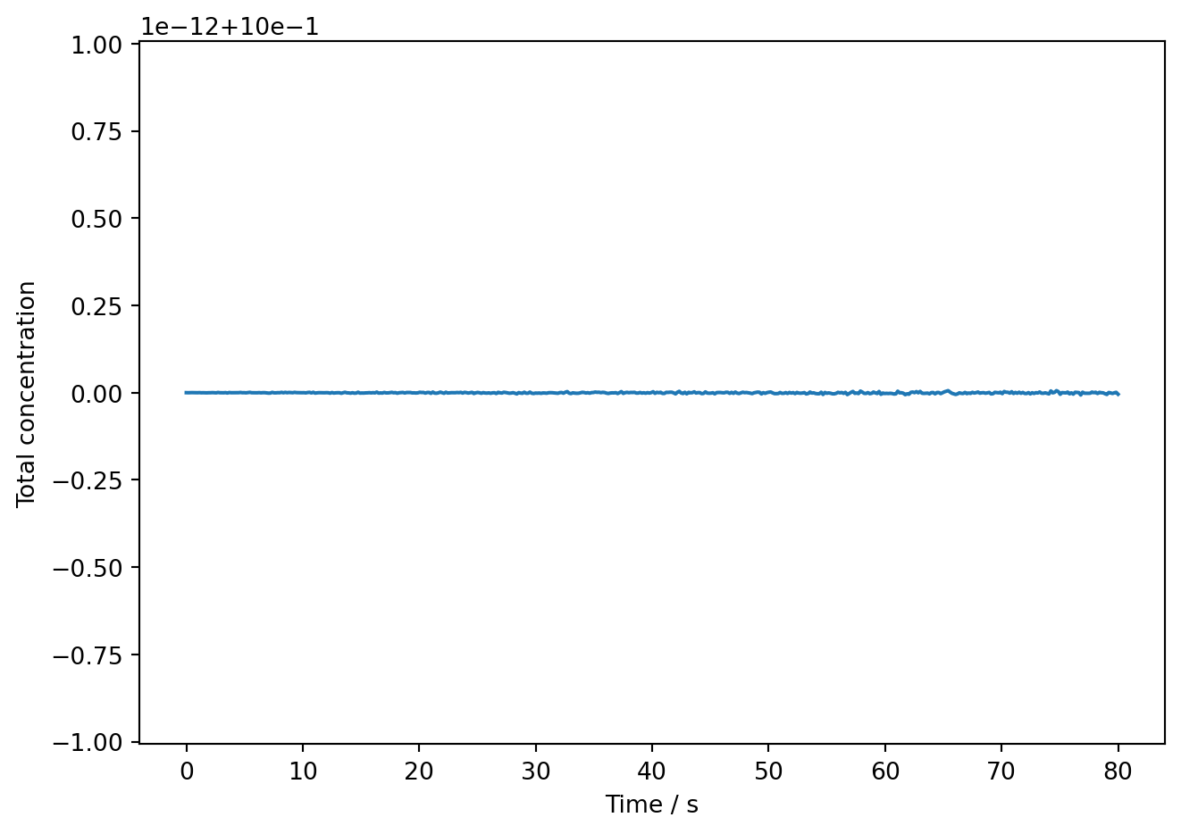
Verify from your plot and numerical results that the total concentration remains constant and that the concentration vector approaches the equilibrium composition found in part c.
Sort the nonzero eigenvalues according to the magnitude of their real parts. The eigenvalue closest to zero describes the slowest decaying mode of the reaction network. Determine its characteristic relaxation time

\[ \tau=-\frac{1}{\operatorname{Re}\lambda}. \]

Compare this value with the time scale over which your numerical solution approaches equilibrium. Explain how the eigenvalues of the rate matrix separate the dynamics of a complicated reaction network into different relaxation time scales.
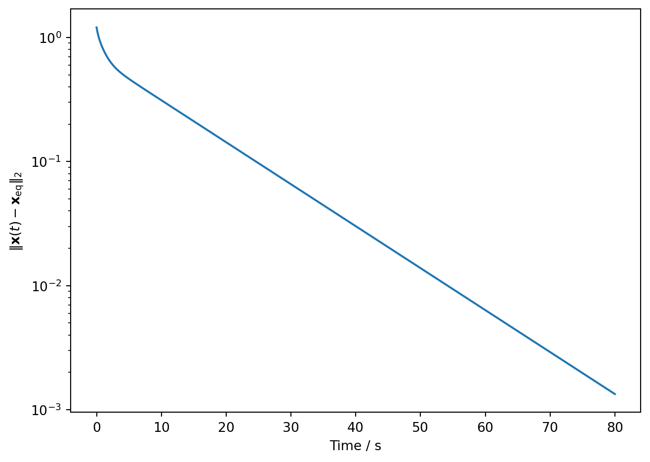
The eigenvalue analysis predicts not only that the system approaches equilibrium, but also how rapidly it does so. Let $\mathbf{x}_{\mathrm{eq}}$ denote the equilibrium concentration vector found in part c, and define the distance from equilibrium by

\[ d(t)=\|\mathbf{x}(t)-\mathbf{x}_{\mathrm{eq}}\|_2. \]

Using your numerical solution from part d, plot $d(t)$ as a function of time using a logarithmic scale for the vertical axis. You can use plt.semilogy for this.

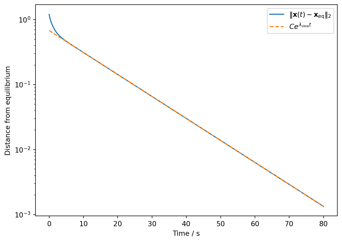
At sufficiently long times, the slowest decaying eigenmode should dominate. If $\lambda_{\mathrm{slow}}$ is the nonzero eigenvalue closest to zero, we therefore expect approximately

\[ d(t)\propto e^{\lambda_{\mathrm{slow}}t}. \]

On the same plot, add a curve proportional to $e^{\lambda_{\mathrm{slow}}t}$, choosing its prefactor so that it can easily be compared with $d(t)$. Do the two curves become parallel at long times? Explain why a straight line on this logarithmic plot provides a direct visualization of the slowest relaxation mode of the reaction network.

Solution for Exercise 9.6

For species A, material is lost through $\mathrm{A}\to\mathrm{B}$ and gained through $\mathrm{B}\to\mathrm{A}$, giving

\[ \frac{da}{dt}=-k_{AB}a+k_{BA}b. \]

Similarly, the remaining rate equations are

\[ \frac{db}{dt}=k_{AB}a-(k_{BA}+k_{BC}+k_{BD})b+k_{CB}c+k_{DB}d, \]

\[ \frac{dc}{dt}=k_{BC}b-k_{CB}c, \]

\[ \frac{dd}{dt}=k_{BD}b-(k_{DB}+k_{DE})d+k_{ED}e, \]

and

\[ \frac{de}{dt}=k_{DE}d-k_{ED}e. \]

Thus,

\[ \frac{d\mathbf{x}}{dt}=K\mathbf{x}, \]

with

\[ K= \begin{bmatrix} -k_{AB} & k_{BA} & 0 & 0 & 0\\ k_{AB} & -(k_{BA}+k_{BC}+k_{BD}) & k_{CB} & k_{DB} & 0\\ 0 & k_{BC} & -k_{CB} & 0 & 0\\ 0 & k_{BD} & 0 & -(k_{DB}+k_{DE}) & k_{ED}\\ 0 & 0 & 0 & k_{DE} & -k_{ED} \end{bmatrix}. \]

With the numerical rate constants, this becomes

\[ K= \begin{bmatrix} -1.0 & 0.4 & 0 & 0 & 0\\ 1.0 & -1.6 & 0.2 & 0.3 & 0\\ 0 & 0.7 & -0.2 & 0 & 0\\ 0 & 0.5 & 0 & -1.1 & 0.1\\ 0 & 0 & 0 & 0.8 & -0.1 \end{bmatrix}. \]

Adding the five rate equations gives

\[ \frac{d}{dt}(a+b+c+d+e)=0. \]

All reaction terms cancel pairwise. Therefore the total concentration

\[ a+b+c+d+e \]

is conserved.

This is also visible from $K$: every column of $K$ sums to zero.

We construct the matrix and diagonalize it numerically.

import numpy as np

kAB = 1.0
kBA = 0.4
kBC = 0.7
kCB = 0.2
kBD = 0.5
kDB = 0.3
kDE = 0.8
kED = 0.1

K = np.array([
    [-kAB,  kBA,                   0.0,             0.0,  0.0],
    [ kAB, -(kBA + kBC + kBD),     kCB,             kDB,  0.0],
    [ 0.0,   kBC,                  -kCB,             0.0,  0.0],
    [ 0.0,   kBD,                   0.0, -(kDB + kDE),  kED],
    [ 0.0,   0.0,                   0.0,             kDE, -kED]
])

print(K)

# Check conservation: the columns should sum to zero
print("Column sums:", K.sum(axis=0))

[[-1.   0.4  0.   0.   0. ]
 [ 1.  -1.6  0.2  0.3  0. ]
 [ 0.   0.7 -0.2  0.   0. ]
 [ 0.   0.5  0.  -1.1  0.1]
 [ 0.   0.   0.   0.8 -0.1]]
Column sums: [ 0.00000000e+00 -2.22044605e-16  0.00000000e+00  0.00000000e+00
  0.00000000e+00]

We now find the eigenvalues and eigenvectors. We sort the eigenvalues from largest to smallest real part so that the eigenvalue closest to zero appears first.

eigenvalues, eigenvectors = np.linalg.eig(K)

order = np.argsort(eigenvalues.real)[::-1]
eigenvalues = eigenvalues[order]
eigenvectors = eigenvectors[:, order]

print("Eigenvalues:")
for value in eigenvalues:
    print(value)

Eigenvalues:
-3.5641539813319436e-17
-0.07786195015156719
-0.6247369441879431
-1.1352737121412337
-2.1621273935192553

Numerically, the eigenvalues are approximately

\[ \lambda= 0,\; -0.07786,\; -0.62474,\; -1.13527,\; -2.16213 \qquad \mathrm{s}^{-1}. \]

The eigenvalue reported by the computer as a number of order $10^{-17}$ should be interpreted as zero; the small deviation from exactly zero is due to floating-point arithmetic.

The zero eigenvalue represents an unchanging mode. This is the equilibrium mode of the reaction network. If

\[ K\mathbf{x}_{\mathrm{eq}}=\mathbf{0}, \]

then

\[ \frac{d\mathbf{x}_{\mathrm{eq}}}{dt}=\mathbf{0}. \]

All the other eigenvalues are negative. A mode with eigenvalue $\lambda<0$ behaves as

\[ e^{\lambda t}, \]

and therefore decays with time. These eigenvalues describe the different ways in which deviations from equilibrium relax.

We identify the eigenvector belonging to the eigenvalue closest to zero and normalize it so that its components sum to one.
```
i0 = np.argmin(np.abs(eigenvalues))

x_eq = eigenvectors[:, i0].real

# Eigenvectors can have an arbitrary overall sign
if x_eq.sum() < 0:
    x_eq = -x_eq

# Normalize to total concentration 1
x_eq = x_eq / x_eq.sum()

print("Equilibrium fractions:")
for species, value in zip(["A", "B", "C", "D", "E"], x_eq):
    print(f"{species}: {value:.6f}")

print("Sum:", x_eq.sum())
```
```
Equilibrium fractions:
A: 0.020101
B: 0.050251
C: 0.175879
D: 0.083752
E: 0.670017
Sum: 1.0
```
This gives approximately

\[ \mathbf{x}_{\mathrm{eq}}= \begin{bmatrix} 0.02010\\ 0.05025\\ 0.17588\\ 0.08375\\ 0.67002 \end{bmatrix}. \]

Thus the equilibrium mixture contains approximately

\[ 2.0\%\ \mathrm{A},\qquad 5.0\%\ \mathrm{B},\qquad 17.6\%\ \mathrm{C},\qquad 8.4\%\ \mathrm{D},\qquad 67.0\%\ \mathrm{E}. \]

The equilibrium vector can also be understood directly from the individual reversible reactions. At equilibrium,

\[ k_{AB}a=k_{BA}b,\qquad k_{BC}b=k_{CB}c,\qquad k_{BD}b=k_{DB}d,\qquad k_{DE}d=k_{ED}e. \]

For example,

\[ \frac{b}{a}=\frac{k_{AB}}{k_{BA}}=\frac{1.0}{0.4}=2.5, \]

and the other equilibrium ratios follow similarly.

We now start with all material in A,

\[ \mathbf{x}(0)= \begin{bmatrix} 1\\0\\0\\0\\0 \end{bmatrix}, \]

and evaluate

\[ \mathbf{x}(t)=e^{Kt}\mathbf{x}(0). \]

Because the slowest relaxation time will turn out to be around $13\ \mathrm{s}$, a time interval of about $0$–$80\ \mathrm{s}$ is sufficient to see the system approach equilibrium.

import matplotlib.pyplot as plt
from scipy.linalg import expm

x0 = np.array([1.0, 0.0, 0.0, 0.0, 0.0])

times = np.linspace(0.0, 80.0, 500)

x_t = np.array([
    expm(K * t) @ x0
    for t in times
])

plt.figure()
for i, species in enumerate(["A", "B", "C", "D", "E"]):
    plt.plot(times, x_t[:, i], label=species)

plt.xlabel("Time / s")
plt.ylabel("Concentration")
plt.legend()
plt.tight_layout()
plt.show()

The plot shows the initial A concentration decreasing while the other species are populated. Eventually all five concentrations become constant and approach the equilibrium fractions found in part c.

We can also check conservation numerically.

total = x_t.sum(axis=1)

print("Minimum total concentration:", total.min())
print("Maximum total concentration:", total.max())
print("Final concentration vector:")
print(x_t[-1])
print("Equilibrium vector:")
print(x_eq)

Minimum total concentration: 0.9999999999999933
Maximum total concentration: 1.0000000000000058
Final concentration vector:
[0.02016436 0.05039847 0.17672309 0.08372369 0.66899039]
Equilibrium vector:
[0.0201005  0.05025126 0.1758794  0.08375209 0.67001675]

A useful visualization of conservation is

plt.figure()
plt.plot(times, total)
plt.xlabel("Time / s")
plt.ylabel("Total concentration")
plt.tight_layout()
plt.show()

Apart from tiny floating-point errors, the total concentration remains exactly $1$.

The nonzero eigenvalue closest to zero is

\[ \lambda_{\mathrm{slow}}\approx -0.07786\ \mathrm{s}^{-1}. \]

Its characteristic relaxation time is therefore

\[ \tau=-\frac{1}{\lambda_{\mathrm{slow}}} \approx\frac{1}{0.07786}\ \mathrm{s} \approx12.84\ \mathrm{s}. \]

We can obtain all the characteristic relaxation times numerically.
```
nonzero = eigenvalues[np.abs(eigenvalues) > 1e-10]

# Sort from slowest to fastest decay
nonzero = nonzero[np.argsort(np.abs(nonzero.real))]

print("Relaxation modes:")
for lam in nonzero:
    tau = -1.0 / lam.real
    print(f"lambda = {lam.real: .6f} 1/s, tau = {tau:.3f} s")
```
```
Relaxation modes:
lambda = -0.077862 1/s, tau = 12.843 s
lambda = -0.624737 1/s, tau = 1.601 s
lambda = -1.135274 1/s, tau = 0.881 s
lambda = -2.162127 1/s, tau = 0.463 s
```
The relaxation times are approximately

\[ 12.84,\qquad 1.60,\qquad 0.88,\qquad 0.46\ \mathrm{s}. \]

Thus the reaction network contains several distinct time scales. Some redistribution takes place very rapidly, while one mode relaxes considerably more slowly.

After a few multiples of the shorter relaxation times, the fast modes have essentially disappeared. The remaining deviation from equilibrium is then dominated by the slow mode,

\[ \mathbf{x}(t)-\mathbf{x}_{\mathrm{eq}} \approx c_{\mathrm{slow}}e^{\lambda_{\mathrm{slow}}t}\mathbf{v}_{\mathrm{slow}}. \]

This illustrates an important use of eigenvalue analysis: a complicated set of coupled rate equations can be decomposed into independent modes with characteristic time scales determined by the eigenvalues.
We now calculate the Euclidean distance from equilibrium,

\[ d(t)=\|\mathbf{x}(t)-\mathbf{x}_{\mathrm{eq}}\|_2. \]
```
distance = np.linalg.norm(x_t - x_eq, axis=1)

plt.figure()
plt.semilogy(times, distance)
plt.xlabel("Time / s")
plt.ylabel(r"$\|\mathbf{x}(t)-\mathbf{x}_{\mathrm{eq}}\|_2$")
plt.tight_layout()
plt.show()
```
The curve becomes approximately straight at long times. To understand this, suppose that only the slowest mode remains. Then

\[ d(t)\propto e^{\lambda_{\mathrm{slow}}t}. \]

Taking the logarithm gives

\[ \log d(t)=\text{constant}+\lambda_{\mathrm{slow}}t. \]

Thus an exponential decay becomes a straight line on a semilogarithmic plot, with slope $\lambda_{\mathrm{slow}}$.

We can compare the numerical distance directly with the predicted slow exponential. We choose a reference time after the faster modes have mostly decayed and set the prefactor so that the two curves agree at that time.
```
lambda_slow = nonzero[0].real

# Choose a reference point in the long-time regime
t_ref = 30.0
i_ref = np.argmin(np.abs(times - t_ref))

# Choose the prefactor so the exponential agrees with d(t)
# at the reference time
prefactor = distance[i_ref] / np.exp(lambda_slow * times[i_ref])
slow_decay = prefactor * np.exp(lambda_slow * times)

plt.figure()
plt.semilogy(
    times,
    distance,
    label=r"$\|\mathbf{x}(t)-\mathbf{x}_{\mathrm{eq}}\|_2$"
)
plt.semilogy(
    times,
    slow_decay,
    "--",
    label=r"$C e^{\lambda_{\mathrm{slow}}t}$"
)

plt.xlabel("Time / s")
plt.ylabel("Distance from equilibrium")
plt.legend()
plt.tight_layout()
plt.show()
```
At early times the two curves need not agree because several eigenmodes contribute simultaneously:

\[ \mathbf{x}(t)-\mathbf{x}_{\mathrm{eq}} = \sum_j c_j e^{\lambda_jt}\mathbf{v}_j. \]

The modes with more negative eigenvalues decay most rapidly. At sufficiently long times, they become negligible compared with the mode whose eigenvalue is closest to zero. Consequently,

\[ \mathbf{x}(t)-\mathbf{x}_{\mathrm{eq}} \approx c_{\mathrm{slow}}e^{\lambda_{\mathrm{slow}}t}\mathbf{v}_{\mathrm{slow}}, \]

and the two curves become parallel on the logarithmic plot.

The numerical dynamics therefore provide a direct visualization of the eigenvalue analysis: the smallest-magnitude nonzero eigenvalue controls the long-time approach to equilibrium.