29 Taylor Series
Taylor series provide one of the most important ways of approximating a smooth function by a polynomial. The central idea is to find a polynomial that approximates the function locally: near a point \(a\), we choose a polynomial whose value and derivatives agree with those of the function at \(a\) up to some order \(n\).
For a sufficiently differentiable function \(f\), the Taylor polynomial of degree \(n\) about \(a\) is
\[ T_n(x)=\sum_{k=0}^n \frac{f^{(k)}(a)}{k!}(x-a)^k. \]
Thus,
\[ T_n(x)=f(a)+f'(a)(x-a)+\frac{f''(a)}{2!}(x-a)^2+\cdots+\frac{f^{(n)}(a)}{n!}(x-a)^n. \]
When \(a=0\), the expansion is called a Maclaurin series. Three particularly important Maclaurin series are
\[ e^x=1+x+\frac{x^2}{2!}+\frac{x^3}{3!}+\cdots, \]
\[ \sin x=x-\frac{x^3}{3!}+\frac{x^5}{5!}-\cdots, \]
and
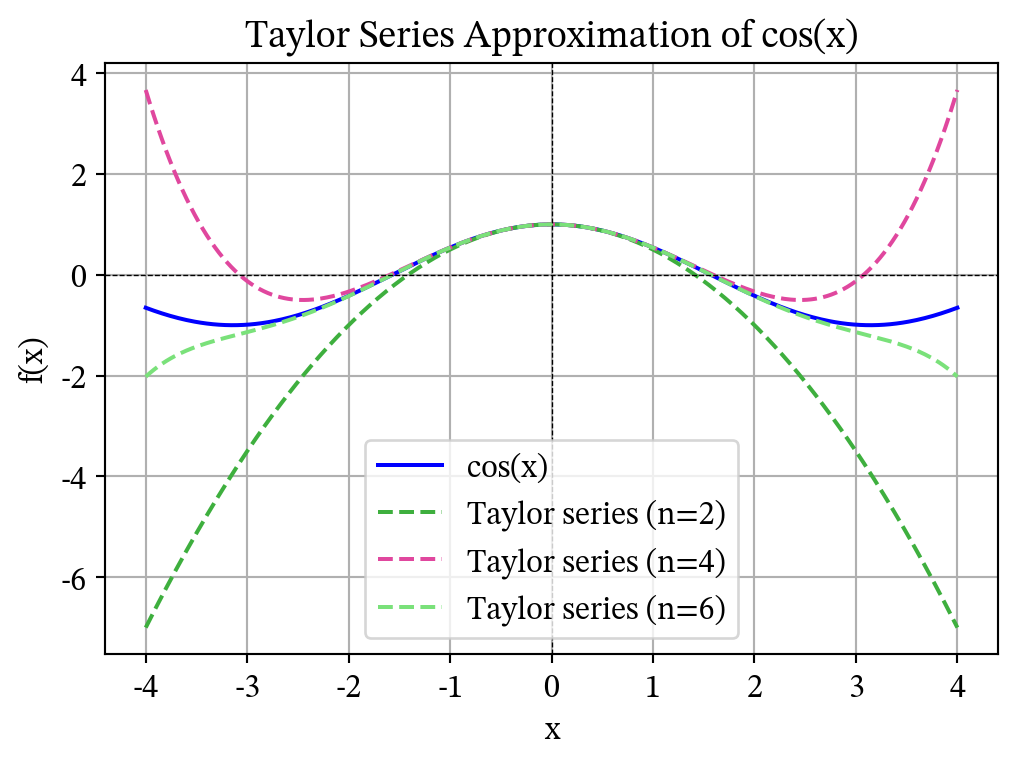
\[ \cos x=1-\frac{x^2}{2!}+\frac{x^4}{4!}-\cdots. \]
Keeping only a few terms gives a low-order approximation. For example, close to \(x=0\),
\[ e^x\approx 1+x,\qquad \sin x\approx x,\qquad \cos x\approx 1-\frac{x^2}{2}. \]
These approximations are local. Thus, they usually become less accurate as we move farther from the expansion point. Increasing the order of the Taylor polynomial generally improves the approximation within a suitable region, but it does not guarantee accuracy far from the expansion point.
The difference between the function and its Taylor polynomial is the remainder,
\[ R_n(x)=f(x)-T_n(x). \]
One useful form is the Lagrange remainder,
\[ R_n(x)=\frac{f^{(n+1)}(\xi)}{(n+1)!}(x-a)^{n+1}, \]
where \(\xi\) lies somewhere between \(a\) and \(x\). Although \(\xi\) is usually unknown, a bound on \(|f^{(n+1)}|\) gives a bound on the error:
\[ |R_n(x)|\leq \frac{M}{(n+1)!}|x-a|^{n+1}, \]
provided \(|f^{(n+1)}(t)|\leq M\) between \(a\) and \(x\).
Taylor series can be generalized to higher dimensions, i.e., functions of several variables.
In molecular physics and quantum chemistry, Taylor expansions appear quite often. An important example is the expansion of a potential-energy function around an equilibrium geometry. Keeping terms only through second order gives the harmonic approximation. Taylor series also extend naturally to functions of matrices and operators, such as the exponential operator.
Exercises
Exercise 29.1 (Approximating the exponential function)
Write down the general Taylor polynomial \(T_n(x)\) about \(x=0\).
For \(f(x)=e^x\), compute \(f(0)\), \(f'(0)\), \(f''(0)\), and \(f'''(0)\).
Construct the Taylor polynomials \(T_1(x)\), \(T_2(x)\), and \(T_3(x)\) for \(e^x\) about \(x=0\).
Use \(T_1\), \(T_2\), and \(T_3\) to approximate \(e^{0.1}\).
Compare your approximations with \(e^{0.1}\approx 1.105170\). Which polynomial gives the best approximation?
Repeat the calculation for \(e^1\). Why are the low-order approximations less accurate at \(x=1\) than at \(x=0.1\)?
Exercise 29.2 (Sine and cosine near the origin)
Compute the first four derivatives of \(f(x)=\sin x\) and evaluate them at \(x=0\).
Use these derivatives to obtain the Taylor polynomial for \(\sin x\) through the cubic term.
Similarly, obtain the Taylor polynomial for \(\cos x\) through the quadratic term.
Use the lowest nonconstant approximations to estimate \(\sin(0.1)\) and \(\cos(0.1)\).
Compare with \(\sin(0.1)\approx0.0998334\) and \(\cos(0.1)\approx0.995004\).
Explain why \(\sin x\approx x\) is called the small-angle approximation. Angles are measured in radians.
Exercise 29.3 (Controlling the error) Consider the Taylor polynomial \(T_n(x)\) for \(e^x\) about \(x=0\).
Write \(T_n(x)\).
Use the Lagrange remainder to show that, for \(0\leq x\leq1\),
\[|R_n(x)|\leq \frac{e}{(n+1)!}x^{n+1}.\]
Find the smallest \(n\) for which this bound guarantees an error below \(10^{-3}\) when approximating \(e^{1/2}\).
Compute the corresponding approximation to \(e^{1/2}\) and compare it with \(e^{1/2}\approx1.64872127\). Compare the actual error with the error bound.
Exercise 29.4 (A Gaussian near its maximum) The Gaussian function \(f(x)=e^{-x^2}\) is closely related to the Gaussian functions used extensively in quantum chemistry.
Starting from the Taylor series for \(e^u\), substitute \(u=-x^2\) and obtain the Taylor polynomial for \(e^{-x^2}\) through order \(x^6\).
Write the quadratic, quartic, and sixth-order approximations explicitly.
Evaluate these three approximations at \(x=0.5\) and compare them with \(e^{-0.25}\approx0.778801\).
Repeat at \(x=1\), where \(e^{-1}\approx0.367879\). What do you observe?
Explain why no finite Taylor polynomial can reproduce the behavior \(e^{-x^2}\to0\) as \(|x|\to\infty\).
Exercise 29.5 (The harmonic approximation) Let \(V(R)\) be the potential energy of a diatomic molecule as a function of the internuclear distance \(R\). Suppose \(R_e\) is an equilibrium bond length and a local minimum of \(V\).
Taylor-expand \(V(R)\) about \(R_e\) through fourth order in the displacement \(q=R-R_e\).
Use the equilibrium condition to simplify the expansion.
Show that retaining terms only through second order gives
\[V(R)\approx V(R_e)+\frac12kq^2,\]
and identify the force constant \(k\).
What physical information is contained in the cubic and quartic terms that is absent from the harmonic approximation?
Consider the Morse potential
\[V(R)=D_e\left(1-e^{-a(R-R_e)}\right)^2.\]
Expand it through fourth order in \(q=R-R_e\) and identify its quadratic, cubic, and quartic coefficients.
Explain qualitatively why the harmonic approximation is expected to work best for small-amplitude vibrations near \(R_e\).
Exercise 29.6 (From the exponential to rotations) Consider the matrix
\[ A=\begin{pmatrix}0&-1\\1&0\end{pmatrix}. \]
The exponential of a matrix is defined by the same power series as the scalar exponential,
\[ e^{\theta A}=I+\theta A+\frac{\theta^2A^2}{2!}+\frac{\theta^3A^3}{3!}+\cdots. \]
Compute \(A^2\), \(A^3\), and \(A^4\), and identify the repeating pattern.
Separate the even and odd powers in the Taylor series for \(e^{\theta A}\).
Recognize the scalar Taylor series that occur and show that
\[e^{\theta A}=I\cos\theta+A\sin\theta.\]
Hence show that
\[e^{\theta A}=\begin{pmatrix}\cos\theta&-\sin\theta\\\sin\theta&\cos\theta\end{pmatrix}.\]
Write approximations to \(e^{\theta A}\) obtained by truncating the exponential series after terms of order \(\theta^2\) and \(\theta^4\).
Explain how this example illustrates the connection between the Taylor series of the exponential, sine, and cosine functions.