11 Measure

We now add the next ingredient: a measure.

Definition 11.1 (Measure, measure space) Let $(X,\mathcal{X})$ be a mesurable space. A measure is a function $\mu : \boldsymbol{X} \to [0,+\infty[ \cup \{+\infty\}$ that satisfies

$\mu(\emptyset) = 0$
For a countable family of disjoint subsets $\{A_i\}\subset \mathcal{X}$, i.e., $A_i\cap A_j = 0$, we have \[\mu\left(\bigcup_i^\infty A_i\right) = \sum_i^\infty \mu(A_i) \qquad\text{$\sigma$-additive}\]

We then say that $(X,\boldsymbol{X},\mu)$ is a measure space.

The definition of the measure $\mu$ encapsulate some intuitive notions about measuring volumes. Volume of nothing is zero, and volume of unions of sets is the sum of the volume. Finally, the infinite union allows for approximation of volumes. Note that a similar idea was present in the definition of the $\sigma$-algebra.

An example that shows how measure can be used differently, consider counting measure:

Example 11.1 (Counting measure) Let $N$ be a finite set, and let $\boldsymbol{N} = 2^N$, the set of all subsets of $N$. This is a $\sigma$-algebra, and since $N$ is finite, we can define counting measure: \[\mu(A) = |A| \quad \text{(number of elements)}\] Having a measure theoretic concept of counting is more useful that one would think! For example, it will allow us to rigorously define square integrable functions over electron configuration space $\mathbb{R}^3 \times \{ \uparrow, \downarrow\}$ in a manner which does not artificially distinguish between discrete and continuous degrees of freedom.

We next introduce the notion of a measurable function. These are functions that we later can define the integral for.

Definition 11.2 (Measurable function) Let $(X,\boldsymbol{X})$ and $(Y,\boldsymbol{Y})$ be measurable spaces. A function \[f : X \to Y\] is called measurable if, for all $U \in \boldsymbol{Y}$, \[f^{-1}[U] \left\{ x \in X \mid f(x) \in U \right\} \in \boldsymbol{X}\]

Note the close analogy with the definition of continuous functions between metric (or more generally topological) spaces: The inverse image of an open set must be open. Measurability of a function is certainly less restrictive: The inverse image of an open set need only be measurable – and we saw that there are “complicated” measurable sets.

Just like for continuous functions, when $f : X \to Y$ with $Y=\mathbb{F}^n$, we get that linear combinations of measurable functions are again measurable. We can also multiply or take absolute values of masurable functions, and still get measurable functions. Perhaps formulate as theorem

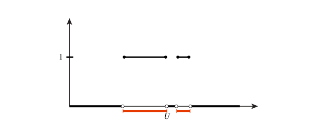
Figure 11.1: Characteristic function of a subset $U$ of $\mathbb{R}$ consisting of two intervals.

Example 11.2 (Example) Why is this a definition that can be useful? Consider the characteristic function $\chi_U$ of some subset $U \subset Y$, defined by \[\chi_U(y) = \begin{cases} 1 & y \in U \\ 0 & y \notin U \end{cases}\] See Figure 11.1. Then the inverse image $\chi_U^{-1}[1]$ is exactly $U$. If $U$ is actually measurable, this means that we can measure it with a measure $\mu : \boldsymbol{Y}\to [0,+\infty[$.

Example 11.3 (Example) Consider the function \[f(x) = \begin{cases} 1 & x \in \mathbb{Q}\\ 0 & x \in \mathbb{R}\setminus \mathbb{Q}\end{cases}\] This function is not Riemann integrable, since the upper and lower Riemann sums will converge to different numbers. However, since $f = \chi_\mathbb{Q}$ we now expect it to be integrable. But what will be the integral? Since $\mu(\mathbb{Q})=0$ we expect that $f^{-1}(1)=\mathbb{Q}$ will not contribute, i.e., the integral is 0.