8 Metric space hierarchy
We are now motivated to look closer at metric spaces, and open and closed sets in metric spaces. In this section, we look at metric spaces, and these will be the most general topological spaces we discuss.
A vector space with a topology is called a topological vector space (TVS).
8.1 Inner product spaces
Definition 8.1 (Inner product) Let \(V\) be a vector space. An inner product \(\left\langle\cdot, \cdot\right\rangle : V\times V \to \mathbb{F}\) is a map which satisfies the following axioms:
\(\left\langle x,x\right\rangle \geq 0\), \(\left\langle x,x\right\rangle = 0\) if and only if \(x = 0\) non-negative
\(\left\langle x,\alpha y + \beta z\right\rangle = \alpha\left\langle x,y\right\rangle + \beta\left\langle x,z\right\rangle\) linearity
\(\left\langle\alpha y + \beta z, x\right\rangle = \bar{\alpha}\left\langle y,x\right\rangle + \bar{\beta}\left\langle z,x\right\rangle\) conjugate linearity
\(\left\langle x,y\right\rangle = \overline{\left\langle y,x\right\rangle}\) hermiticity
We say that the pair \((V,\left\langle\cdot,\cdot\right\rangle)\) is an inner-product space.
8.2 Normed spaces
In Euclidean space, the length of a vector \(\mathbf{v}\in\mathbb{F}^n\) is \(\|\mathbf{v}\| = \sqrt{\left\langle\mathbf{v},\mathbf{v}\right\rangle}\). This is but one out of many possible norms on Euclidean space. Norms are abstractions of the notions of length of elements of vector spaces:
Definition 8.2 (Norm) Let \(V\) be a vector space. A norm \(\|\cdot\| : V \to \mathbb{R}_+ = [0, +\infty[\) is a function that satisfies the following axioms:
\(\|x\| \geq 0\), and \(\|x\|=0\) if and only if \(x = 0\). positivity
\(\|\alpha x\| = |\alpha| \|x\|\) absolute homogeneity
\(\|x + y \| \leq \|x\| + \|y\|\) triangle inequality
The pair \((V,\|\cdot\|)\) is called a normed vector space.
You should convince yourself that the axioms indeed correspond to what we expect from a useful concept of length.
8.3 Angles between vectors
Returning to the inner product, we can now obtain some intuition using the associated norm. The inner product measures angles between vectors. Indeed, any inner product satisfies the Cauchy–Schwarz inequality:
Lemma 8.1 (Cauchy–Schwarz inequality) Let \((V,\left\langle\cdot,\cdot\right\rangle)\) be an inner product space, and let \(\|\cdot\|\) be the induced norm. Then, for any \(x,y \in V\), it holds that \[\left\langle x,y\right\rangle \leq \left\langle x,x\right\rangle^{1/2} \left\langle y,y\right\rangle^{1/2} = \|x\|\, \|y\|.\]
The Cauchy–Schwarz inequality implies that \[0 \leq \frac{|\left\langle x,y\right\rangle|}{\|x\|y\|} \leq 1\] so that we may define the angle between the vectors as the unique \(\theta \in [0,\pi/2]\) such that \[\cos \theta = \frac{|\left\langle x,y\right\rangle|}{\|x\|\|y\|}.\] Note in particular that if \(\left\langle x,y\right\rangle=0\), then \(\theta = \pi/2\), coinciding with the notion of \(x\) and \(y\) being orthogonal to each other.
8.4 Metric spaces
Norms can be used to measure distance in Euclidean space and in inner product spaces in general. Given two elements \(\mathbf{u},\mathbf{v}\in\mathbb{F}^n\), the distance is given by \(\|\mathbf{u}-\mathbf{v}\|\). This is a special case of a metric, whose definition gives axioms that encapsulate the notion of distance:
Definition 8.3 (Metric) Let \(M\) be a set. A function \(f: S\times S \to \mathbb{R}\) is a metric if it satisfies the following axioms:
\(d(x,y) = d(y,x)\) symmetry
\(d(x,y) \geq 0\), and \(d(x,y) = 0\) if and only if \(x =y\) positivity and nondegeneracy
\(d(x,y) \leq d(x,z) + d(z,y)\) triangle inequality
The pair \((M,d)\) is a metric space. If \(M\) is a vector space, we say that \((M,d)\) is a metric vector space.
In this definition, note that we are not starting with a vector space, since none of the axioms actually use vector space properties of the set!
Again, make sure that you understand how the axioms embody essential properties expected from a distance measure.
8.5 The topology generated by a metric
Let a metric space \((M,d)\) be given. The metric can be used to define a topology in terms of open balls:
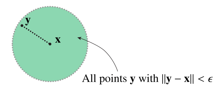
Definition 8.4 (\(\epsilon\)-ball) Let \((M,d)\) be a metric space. Let \(x \in M\). The \(\epsilon\)-ball around \(x\) is the set \[B_\epsilon(x) = \{ y \in M \mid d(x,y) < \epsilon \}.\]
The following definition contains some statements that need to be proven, but we will take them for granted:
Definition 8.5 (Metric space topology) Let \((M,d)\) be a metric space. The metric space topology is the smallest topology \(\tau\) on \(M\) that contains all the open balls. It is the topology generated by the open balls. Every open set in \(\tau\) can be written as an arbitrary union of open balls.
Thus, the \(\epsilon\)-ball is the archetypal open set in a metric space \(M\), and an open ball is illustrated in Figure 8.1.
There are usually many different possible metrics. Sometimes these give different topologies, sometimes the same. In the next example, we give two common metrics on \(\mathbb{R}^2\). It is a fact that these metrics give rise to the same topologies!
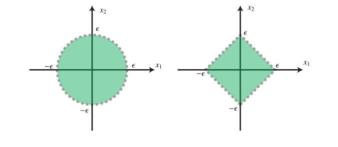
Example 8.1 (Two metrics on \(\mathbb{R}^2\)) Let us consider \(\mathbb{R}^2\) with the usual Euclidean metric. Denote by \(\mathbf{x} = (x_1,x_2)\) and \(\mathbf{y} = (y_1,y_2)\) two points in \(\mathbb{R}^2\). Then the Euclidean distance between these points is \[d_{\text{Euclidean}} (\mathbf{x}, \mathbf{y}) = [(x_1-y_1)^2 + (x_2-y_2)^2]^{1/2}.\] Furthermore, the open ball of radius \(r\) around the origin is the set \[B_\epsilon(0, \text{Euclidean}) = \left\{ (x,y) \in \mathbb{R}^2 \mid x^2 + y^2 < \epsilon^2 \right\}.\] This is the geometric description of the interior of a circle with radius \(\epsilon\) centered at the origin.
Let us consider an alternative metric, the Manhattan metric, named so because it is the relevant metric from the point of view of a taxicab driving along perfectly straight streets that cross each other at right angles: \[d_{\text{Manhattan}}(\mathbf{x}, \mathbf{y}) = |x_1-y_1| + |x_2-y_2|.\] The open ball of raius \(\epsilon\) around the origin is now: \[B_\epsilon(0, \text{Manhattan}) = \left\{ (x,y) \in \mathbb{R}^2 \mid |x| + |y| < \epsilon \right\}.\]
The Euclidean \(\epsilon\)-ball is illustrated below to the left, while the Manhattan unit ball is illustrated to the right:
It is common to use the following characterization as the definition of open sets in vector calculus.
Theorem 8.1 (Characterization of open sets) Let \((M,d)\) be a metric space. A subset \(S\subset M\) is open if and only if for every \(x\in S\) there is an \(\epsilon>0\) such that \(B_\epsilon(x) \subset S\).
The definition of open sets can be used to define the following intuitive notions:
Definition 8.6 (Boundary and interior) Let \((M,d)\) be a metric space, and let \(A \subset M\) be any y subset.
A point \(x\in A\) is called a boundary point if for all \(\epsilom>0\), \(B_\epsilon(x)\) contains a point in \(A\) and a point in \(A^\complement\).
The boundary \(\partial A\) is the set of boundary points of \(A\).
The interior of \(A\) is the set of all points \(x\in A\) such that for some \(\epsilon>0\), \(B_\epsilon(x) \subset A\).
The closure of \(A\) is the smallest closed set containing \(A\), and is equal to \(A \cup \partial A\). (The latter statement is a theorem, not a definition.)
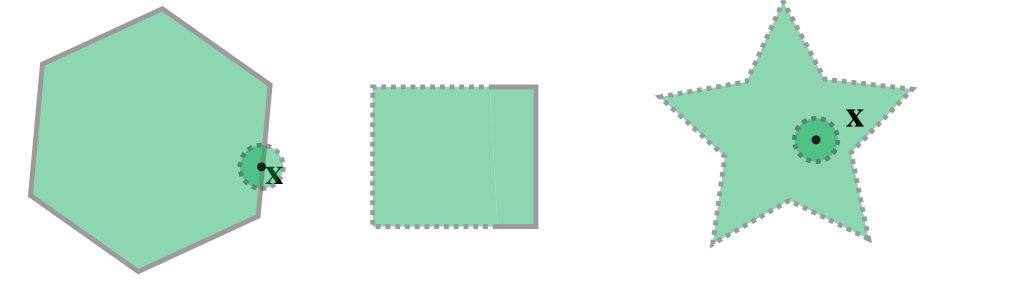
In Figure 8.2 subsets that are open, closed, and neither open nor closed are illustrated. The reason why we can conclude easily about openness and closedness is that from the above example and definition, open sets do not contain their boundaries, while closed sets to.
Example 8.2 (The open ball and its boundary) Consider the open ball \(B_\epsilon(x)\), \[B_\epsilon(x) = \{ y \in M \mid d(x,y) < \epsilon \} .\] Since this set is open, the interior is the set itself. The boundary of the ball is given by \[\partial B_\epsilon(x) = \{ y \in M \mid d(x,y) = \epsilon \} .\] The closure of the ball is \[\operatorname{cl}B_\epsilon(x) = \{ y \in M \mid d(x,y) \leq \epsilon \} .\]